Usage

Installation

It is recommended you use voxelmap through a virtual environment. You may follow the below simple protocol to create the virtual environment, run it, and install the package there:

$ virtualenv venv
$ source venv/bin/activate
(.venv) $ pip install tensorscout

To exit the virtual environment, simply type deactivate. To access it at any other time again, enter with the above source command.

Splitting Sampling Tasks Across Multiple Processors

When performing Monte Carlo sampling at a high number, it can significantly impact computing power. To address this, we have developed the @multicarlo decorator, which allocates a specific number of iterations to a defined number of available processors or cores. In our case, since we have a computer with 4 cores, we have set the num_cores to 4. However, you can set it to as many cores as your computer or server may have available.

In this example, we compare the runtime performance of this multiprocessing decorator with the bare approach, which uses a single core. We begin by importing all the required modules and defining a function that is used in both approaches to avoid redundancy.

import tensorscout as scout
import numpy as np
import matplotlib.pyplot as plt
from timethis import timethis

def make_histograms(data,results, title):
   plt.figure()
   plt.title(title+' N = 100,000')
   plt.hist(data,bins = 7, alpha=0.5,label='data')
   plt.hist(results,bins=600,alpha=0.5,color='magenta',label='data resampling')
   plt.legend()

print()
data = np.random.normal(0, 1, 1000)

The operations we run on both methodologies are random sampling operations which take random numbers from the data distribution defined above, which is a distribution made from 1,000 samples from a Gaussian distribution with a mean of 0 and standard deviation of 1. For both methods, we set the number of samples to 100,000, which is a considerable amount. In the following code block, we apply the @multicarlo decorator to our random sampling function monte_carlo_function and distribute the sampling iterations across four cores.

The timethis() function is used to record the run times of both methods and print them as a terminal output.

title = 'data resampling (with @multicarlo -- 4 cores)'
with timethis(title):
   @scout.multicarlo(num_iters=100000, num_cores=4)
   def monte_carlo_function(data, *args, **kwargs):
      simulated_data = np.random.normal(np.mean(data), np.std(data))
      return simulated_data

   results = monte_carlo_function(data)
   print('number unique results: {}/{}'.format(len(np.unique(results)),len(results)))

   make_histograms(data,results,title)

print('...........................................................')

The following code block executes the same tasks as the previous block, but using a bare approach, meaning that it uses a single core to perform all 100,000 random samples.

title='data resampling (bare)'
with timethis(title):

   def monte_carlo_function_bare(data, *args, **kwargs):
      simulated_data = np.random.normal(np.mean(data), np.std(data))
      return simulated_data

   results = [monte_carlo_function_bare(data) for i in range(100000)]
   print('number unique results: {}/{}'.format(len(np.unique(results)),len(results)))
   make_histograms(data,results,title)

#make plots for both approaches
plt.show()

The output for the previous three code blocks is displayed below.

>>> [OUT]
number unique results: 100000/100000
data resampling (with @multicarlo -- 4 cores): 3.726 seconds
...........................................................
number unique results: 100000/100000
data resampling (bare): 6.478 seconds

We compared multiprocessing and naive methods for generating random numbers and tracked the number of unique results. This showed that multiprocessing generated unique random numbers across different cores. Both methods produced similar random sampling distributions, but the multiprocessing approach using @multicarlo with 4 cores showed around a runtime improvement of 170% over the bare approach.

Campfire

Mapping and Storage of Large and Structurally-Diverse Results with Parallel Computing

Campfire is a powerful tool designed to enable multiprocessing of tests and simulations. It operates on the basis of generating a Python dictionary as output for each simulation that is run. These dictionaries contain the results of each simulation and are split across multiple CPU cores for processing.

Once the simulations have completed, Campfire then collects the dictionaries from all of the simulations and rebuilds them into a single, parent dictionary. This parent dictionary contains all of the results from the individual simulations and is designed to make it easy for users to analyze and interpret the data generated by their simulations.

Campfire is a valuable tool for anyone working with complex simulations or large data sets, as it can greatly accelerate the speed at which simulations are run and analyzed. Its use of Python dictionaries as output provides users with a high degree of flexibility and adaptability to a wide range of different simulation and testing scenarios.

Campfire can be a more powerful decorator than Multicarlo because dictionaries can return several outputs and may be accessed by their keys. The below example is from the Python tests section and shows how to return values from a “simulation” stored in x y z keys.

def unique(key='x'): return len(np.unique(map[key]))

with timethis("Campfire dictionary"):

   @scout.campfire(num_iters=400, num_cores=4)
   def simulation(data):
      for i in range(1000):
            'the above 1,000 iters is to stress-test  the campfire method against the bare (no multiproc) method (in the end, only the last samples from x y and z are returned)'
            x = [np.random.normal(0, 1) for i in range(5)]
            y = [np.random.normal(0, 1) for i in range(5)]
            z = [np.random.normal(0, 1) for i in range(5)]

      return {'x': x, 'y': y, 'z': z}

   data = 'c'
   map = simulation(data)
   print('unique samples -- x: {}, y: {}, z: {}'.format(unique('x'),unique('y'),unique('z')) )

print('...................................................')

with timethis("bare dictionary"):

   def simulation_bare(data, num_iters):
      X,Y,Z = [],[],[]
      for j in range(num_iters):
            for i in range(1000):
               x = [np.random.normal(0, 1) for i in range(5)]
               y = [np.random.normal(0, 1) for i in range(5)]
               z = [np.random.normal(0, 1) for i in range(5)]
            X.extend(x), Y.extend(y), Z.extend(z)

      return {'x': X, 'y': Y, 'z': Z}

   data = 100
   map_bare = simulation_bare(data, num_iters=400)
   print('unique samples -- x: {}, y: {}, z: {}'.format(unique('x'),unique('y'),unique('z')) )

>>> [OUT]
unique samples -- x: 2000, y: 2000, z: 2000
campfire dictionary: 3.013 seconds
...................................................
unique samples -- x: 2000, y: 2000, z: 2000
bare dictionary: 5.421 seconds

Notice how much additional scripting is needed to re-organize the data with simulations on a bare (no Campfire) dictionary. Below we compare the 2000 x,y,z entries graphically between the Campfire sampling and the naive bare sampling from above.

Simulations with Campfire (left) and with a naive bare approach (right). The above were drawn with the voxelmap draw method for coordinates from the voxelmap package

Cakerun: Parallel Computing on Split Matrices

The question of whether it’s faster to eat a cake alone or have 100 people cut a slice and eat their portions until it’s gone highlights the main concept behind the cakerun decorator. Essentially, the decorator partitions an array into a specified number of equally-sized sectors and performs the same task on all sectors in parallel.

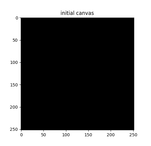
In this example, we set the number of cores to 4 and compare the performance of using multiprocessing versus using a single core. Before proceeding, we import all necessary modules and define the draw function which is used in both approaches to avoid redundancy. Additionally, we define the initial matrix, which is a 252 x 252 matrix of 1s, that will be operated on by both methodologies.

import tensorscout as scout
import numpy as np
import matplotlib.pyplot as plt
from timethis import timethis

num_iters = 40000

def draw(result):
   plt.figure()
   plt.title('{} -- $N_{{perforated}}$ = {}'.format(title, np.multiply(*result.shape) - np.count_nonzero(result)))
   plt.imshow(result,cmap='bone')


matrix = np.ones((252,252))

plt.imshow(matrix,cmap='bone')
plt.title('initial canvas')

In this example, the initial matrix is composed entirely of 1s and will appear as a single color when drawn. The purpose of this code is to apply an operation called “perforation” to the matrix. At each iteration, a random x-y coordinate is selected and the value at that location is set to 0.

The first case demonstrates the use of the @cakerun decorator to split the matrix into sectors and apply the perforate function to each sector. The former code block specifies 40,000 perforating iterations, which for the case of this aprroach has them evenly distributed across the 4 sectors, resulting in 10,000 iterations per sector, ocurring simultaneously.

title = 'cakerun MP (4 cores)'
with timethis("{}".format(title)):

   cores = 4
   @scout.cakerun(num_cores=cores, L_sectors=2)
   def perforate(sector):

      for i in range(num_iters // cores):
            cds = np.argwhere(sector!=0)
            sector[tuple(cds[np.random.randint(cds.shape[0])])] = 0
      return sector

   result = perforate(matrix)
   draw(result)

In the next code block, the perforating operation is applied for 40,000 iterations using a bare approach with a single processor. Hence, there is no task split involved.

title = 'single core'
with timethis("{}".format(title)):

   def perforate_bare(sector):
      for i in range(num_iters):
            cds = np.argwhere(sector!=0)
            sector[tuple(cds[np.random.randint(cds.shape[0])])] = 0
      return sector


   result = perforate_bare(matrix)
   draw(result)


plt.show()

The following are graphical and runtime comparisons of both methods:

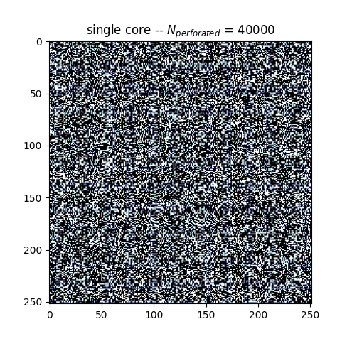
>>> [OUT]
cakerun MP (4 cores): 2.968 seconds
single core: 25.868 seconds

It is apparent that both approaches yield a similar outcome and have the same number of perforations. However, the @cakerun decorated function, which uses four cores simultaneously, has a runtime that is 8-9 times faster than the bare approach.